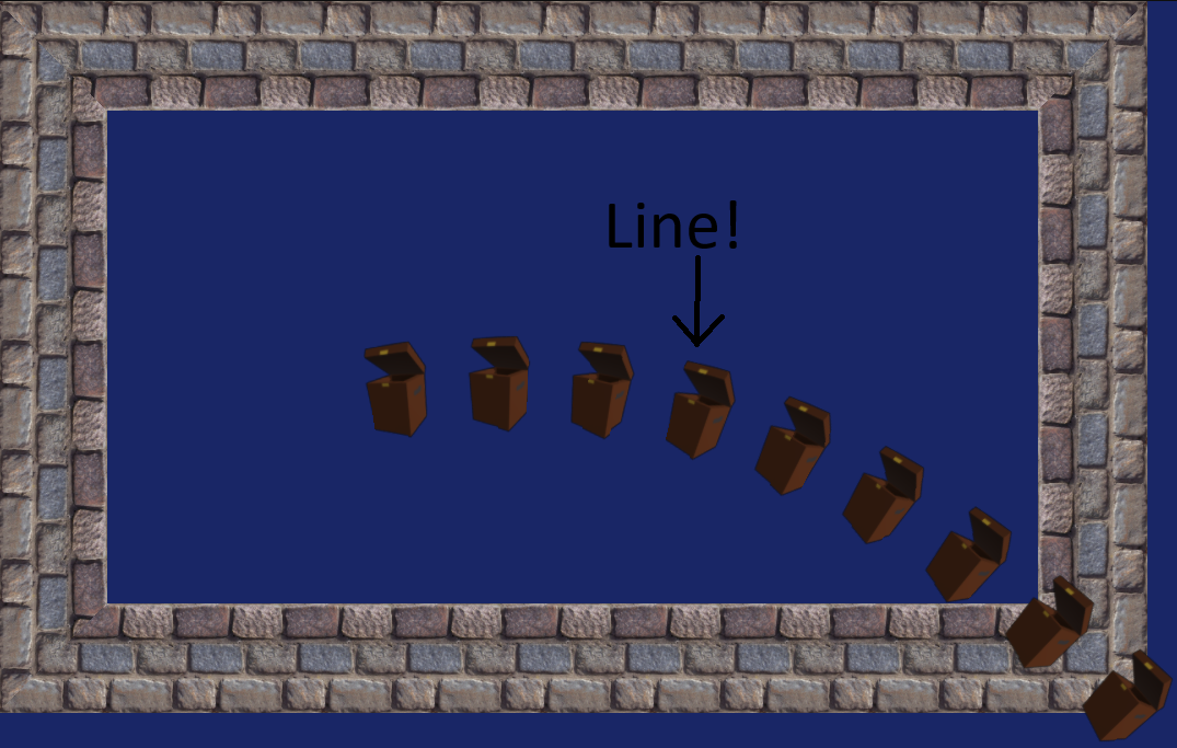
Intro
Lines are a fundamental rendering primitive so drawing them must be easy, right?
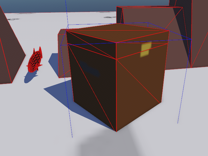
Correct! Drawing lines is easy! Graphics APIs, like Vulkan and OpenGL, expose line topologies so lines can be drawn just like triangles. Changing the line width is as easy as glLineWidth(10.0f).
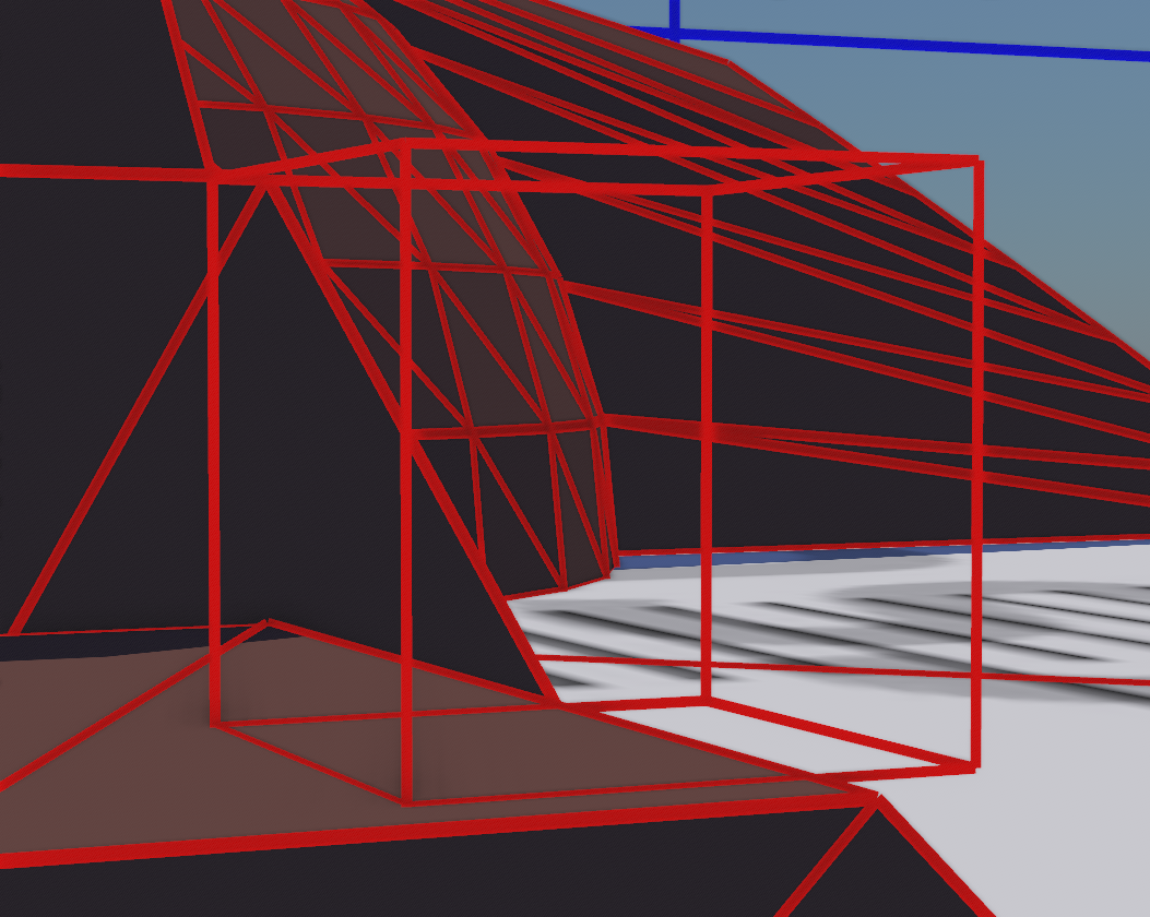
But this brings us to our first, and most obvious problem. The width of these lines is calculated in screen space; Lines further away are the same width as those close to the camera. The second major problem is easy to miss but once you notice, you don’t stop noticing.

See that? The lines don’t properly join up with eachother. Surely the graphics APIs have an easy solution to this?
Nope. We’ve hit the limit of line primitives. Actually, the limit was at glLineWidth depending on your hardware. The OpenGL standard only guarentees that 1.0f is supported. So how do we solve these issues?
Hello Line
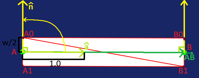
Starting out we’re going to draw a simple line from A to B with a fixed width. To do so we need to generate a rectangle mesh. The vertices will be located width / 2 units away along the line normal in both directions. Mathematically that looks like:
$$ \vec{a} = B - A \hspace{1cm} \hat{a} = \frac{\vec{a}}{\|\vec{a}\|} \hspace{1cm} \hat{n} = \begin{pmatrix} 0 & 1 \\ -1 & 0\end{pmatrix} \hat{a} $$ $$\vec{o} = \hat{n} * \frac{w}{2}$$ $$ A_{0}= A + \vec{o} \hspace{1cm} A_{1}= A - \vec{o}\\ B_{0}= B + \vec{o} \hspace{1cm} B_{1}= B - \vec{o} $$
Visually:
Programmatically:
vec2 AB = B - A;
vec2 direction = normalize(AB);
vec2 normal = vec2(-direction.y, direction.x);

vec2 offset = normal * width / 2.0f;

vec2 A0 = A + offset;
vec2 A1 = A - offset;
vec2 B0 = B + offset;
vec2 B1 = B - offset;
You might’ve noticed that if A and B are the same point we’ll end up dividing by zero. There are several ways to handle this, the simplest and most common solution is to not draw the line at all.
We can repeat this process for each pair of points to get more complex lines, essentially getting us back to the line primitives. (I’ll leave projection into 3D space as an exercise for the reader)
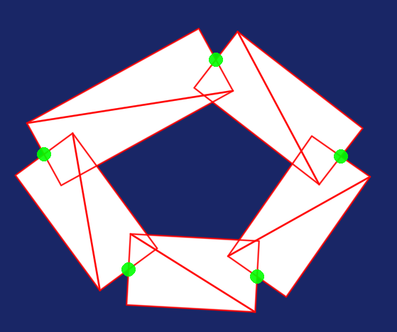
One thing I didn’t mention was the issue of anti-aliasing. The graphics API images in the intro used 4xMSAA, the new images have no MSAA but they look very clean. To achieve this I’m using an anti-aliasing technique that relies on our next topic, assigning UVs.
UV Mapping
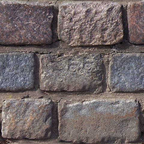
In my research for this article I noticed most articles avoid this topic despite its importance. There are tons of ways to assign UVs, some more complex than others. I’ll be using the following texture (sourced from here) to show the effects.
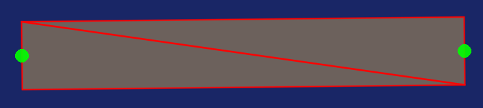
Constant UVs
This is the simplest mapping, give each vertex the same UVs and that’s it. The result is a solid color across the whole line.
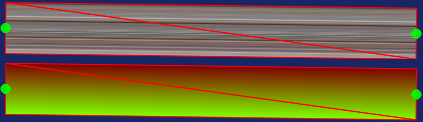
A more interesting technique is to have a constant U but have V at 1.0 on one side of the line and 0.0 on the other. Which side you choose determines the orientation of the texture. The result of this is the texture U stretched across the entire line. For UV visualization the red channel is U and green is V. I have V = 1.0 on the bottom.
Distance UVs
Setting V to [0.0, 1.0] is useful but a slightly more useful technique is to set V on the edges to -1.0 and 1.0. This effectively gives us a V value that represents our distance from the center line. We can remap this to [0.0, 1.0] for texturing and visualization with (V + 1.0) / 2.0 (In fact I was already doing this). We can use this for styling and techniques like anti-aliasing. Here I’m changing the alpha by smoothstep(1.0, 0.0, abs(V)). This effect is possible with [0.0, 1.0] but for more complex lines [-1.0, 1.0] simplifies some math.

That leaves us with U, what do we do with U? There are many, many, many, things you can do with U. Each give a different effect and have their uses, here are some for inspiration.
Line Count
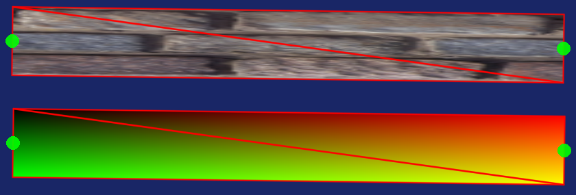
A simple but effective technique is the have U represent where on the current line you are. To do so the left vertices will have a U of n and the right vertices will be n + 1. This streches the texture across the length of the line like so.
True Distance
Another technique is to use the world space distance along the line as the U. Usually a scaling factor is also used to control how fast the texture tiles. For a square texture like this I use 1.0 / line_width as the scaling factor. The result is pleasant.
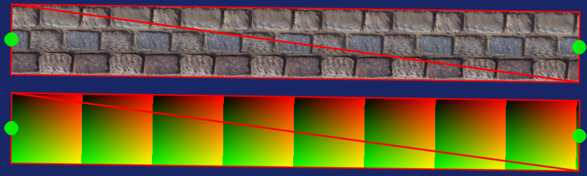
One thing I left purposely vague was where the distance comes from. For a single line segment we can use the distance from A to B or even the distances between the vertices. But things get significantly more complex once we start joining lines together.
Joins
Miter
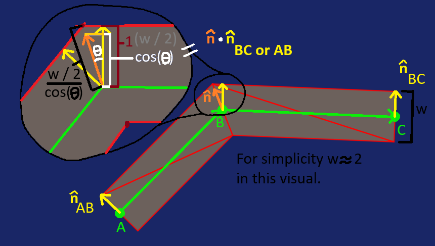
Miter joins are a simple yet effective way to connect line segments. To calculate the direction we add the normals of AB and BC then normalize. The magnitude is a bit trickier but nothing crazy. Our goal is to get the dot product between both of the segment normals and join normal (with magnitude) to equal 1. We start by doing a dot product between the new normal and either of the segment normals, this projects the new normal onto the segment normal telling us how far off of 1 we are. Ignoring width, this means our magnitude is the reciprocal of the dot product. Since everything is now 1 based we can multiply by half the width to get the final magnitude. Apply this direction and magnitude to the point B and that gives us the join locations.
Mathematically: $$ \vec{ab} = B - A \hspace{1cm} \hat{ab} = \frac{\vec{ab}}{\|\vec{ab}\|} \hspace{1cm} \vec{bc} = C - B \hspace{1cm} \hat{bc} = \frac{\vec{bc}}{\|\vec{bc}\|} $$ $$ \hat{n_{ab}} = \begin{pmatrix} 0 & 1 \\ -1 & 0\end{pmatrix} \hat{ab} \hspace{1cm} \hat{n_{bc}} = \begin{pmatrix} 0 & 1 \\ -1 & 0\end{pmatrix} \hat{bc} $$ $$ \vec{n} = \hat{n_{ab}} + \hat{n_{bc}} \hspace{1cm} \hat{n} = \frac{\vec{n}}{\|\vec{n}\|} $$ $$ m = \frac{w / 2}{\hat{n} \cdot \hat{n_{ab}}} $$ $$ B_0 = B + \hat{n} * m \hspace{1cm} B_1 = B - \hat{n} * m $$
Visually:
Programatically:
vec2 AB = B - A;
vec2 BC = C - B;
vec2 normal_AB = normalize(vec2(-AB.y, AB.x));
vec2 normal_BC = normalize(vec2(-BC.y, BC.x));
vec2 new_normal = normalize(normal_AB + normal_BC);

// = cos(θ) ;)
float projection = dot(normal_AB, new_normal);
vec2 join = new_normal * (width / 2.0f) / projection;

vec2 B0 = B + join;
vec2 B1 = B - join;
We’ve corrected the positions but depending on our UVs we might need to correct those. The true distance U values have become stretched and warped.
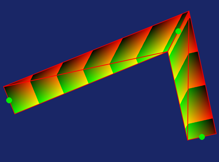
There is no correct solution for this, you will always have some form of stretching or discontinuity. My personal solution is to introduce a discontinuty at the join but eliminate all stretching. For this the distance A0 -> B0 and A1 -> B1 is used for the AB vertices at B. For the BC vertices the outer vertex uses the AB distance for that vertex. The inner vertex uses the outer vertex distance plus the projection of the inner vertex onto BC.
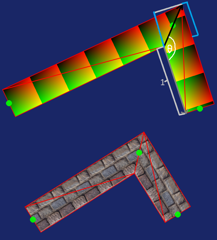
I won’t go over the math in detail, this is more of a proof of concept, I’m still figuring out if I like this solution or not. Regardless, miter joins have a huge problem. Sharp angles look extremely bad.
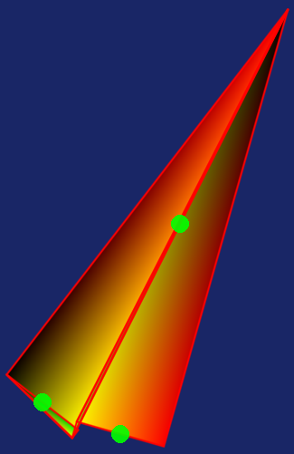
A solution to this problem is if projection (the dot product from calculating the miter earlier) is less than some threshold use a different type of join for the outer edge. Such as the bevel join.
Bevel
The bevel join reuses a lot of the math from the miter join but only applies it to the inner vertex. Unlike the miter, it adds new geometry to the mesh, a triangle between the outer vertices and the inner one. The only new math we need is how to determine which vertex is inner or outer. For this I use the sign of the dot product between BC and the normal of AC.
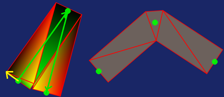
As you can see, the bevel join handles sharp angles much better. Correcting the UVs is a bit different but I didn’t bother working out the math. Unfortunately, I don’t find bevels very interesting or appealing so I’m not going to spend much time on them.
Round
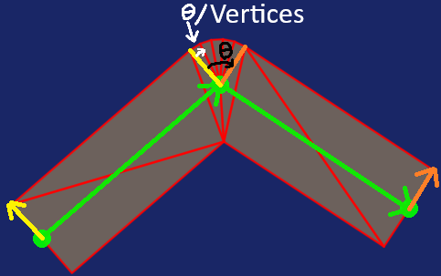
The round is similar to the bevel in that it creates new geometry and is safe as the outer join. However, unlike the bevel it requires new vertices. The ideal topology uses the inner join vertex and outer vertices directly for the triangles. However, this causes issues with UVs, so we’re going to add an extra vertex and two triangles to get correct V values.
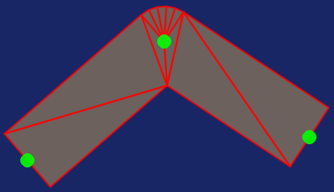
One thing of note is the amount of new vertices we need. For this I have a parameter specifying the degrees per vertex, but you could also used a fixed amount. Regardless of technique, knowing the degrees the join spans is an important part of the math. We can take advantage of the geometric form of the dot product to calculate this. In specific, taking the arccos of the segment normals gives us the degrees we’ll be spaning. I use an iterative approach to calculate the new vertices. Starting at the normal of AB each vertex is calculated as B + direction * (width / 2) (changing sign depending on where the outer edge is). Then direction is rotated by theta / new_vertex_count and the process gets repeated.
Mathematically: $$ s = -\frac{\hat{n_{ab}} \cdot \vec{bc}}{|\hat{n_{ab}} \cdot \vec{bc}|} $$ $$ \theta = \cos^{-1}({\hat{n_{ab}} \cdot \hat{n_{bc}}})\hspace{1cm} v = \lfloor \frac{\theta^\circ}{p} \rfloor + 1 \hspace{1cm} \Delta\theta = \frac{\theta}{v} * s $$ $$ \mathbf{R} = \begin{pmatrix} \cos{\Delta\theta} & -\sin{\Delta\theta} \\ sin{\Delta\theta} & \cos{\Delta\theta}\end{pmatrix} $$ $$ \hat{d_0} = \mathbf{R} \hat{n_{ab}} \hspace{1cm} \hat{d_n} = \mathbf{R} \hat{d_{n-1}} $$ $$ m = \frac{w}{2} * s \hspace{1cm} V_n = B + \hat{d_n} * m $$
Visually:
Programatically:
float inner_outer = -sign(dot(normal_AB, BC));
float theta = acos(dot(normal_AB, normal_BC));

// note the radians to degrees conversion
int new_vertex_count = floor(degrees(theta) / degrees_per_vertex) + 1;

float delta_theta = theta / new_vertex_count * inner_outer;
mat2 rotation_matrix {
    cos(delta_theta), -sin(delta_theta),
    sin(delta_theta), cos(delta_theta)
};

vec2 direction = normal_AB;
for (int i = 0; i < new_vertex_count; ++i) {
    direction = rotation_matrix * direction;
    vec2 Vi = B + direction * (width / 2.0f) * inner_outer;
}
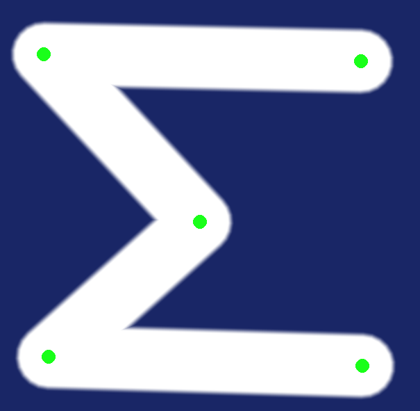
With this we’ve covered the main 3 types of joins, but we’re still missing a critical part of the line drawing process. See if you can spot what I added here:
Ends
Line ends are the final piece in our linear puzzle. The math behind these is much simpler since we only need a point and a direction. Depending on your application not having ends can also look good. These are less important than joins but still important in design.
Square
The square end style takes the ending vertices and extrudes them outwards by half the width.
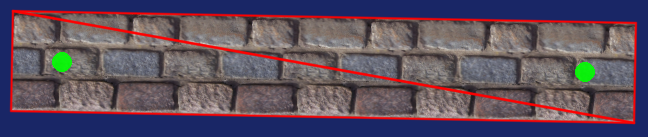
The geometry I used does not preserve V as the distance on the ends. To fix V we’d need to add a vertex at the endpoint and introduce a discontinuity when V switches between -1 and 1. But it looks good either way.
Round
The round end style is very similar to the round join, in fact the math (and code) are almost identical. Instead of rotating the normal between itself and the joining normal, the final direction will always be 180 degrees away. With how we triangulated the round join earlier we will have the correct V too.

If you look closely (top right or bottom left) you can see the discontinuity of V when it switches between -1.0 and 1.0. This would look worse on a textured line but I find rounds most useful for less structured lines anyways.
Closing
With this we can now draw beautiful, anti-aliased, textured, colored lines. That was a lot, and trust me, we’re still only touching the surface. There is a lot more to line drawing than connecting points. Figuring out what points to connect and how to do so efficiently is a huge part of it.
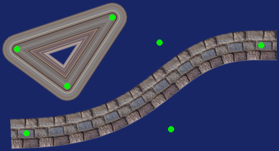
With that I leave you with this; a strange shape floating above a cubic bézier curve.
References
*I don’t use Unity but the concepts are transferable